Combined

General

Sets of Numbers

Sets

Symbol	Description
$\mathbb{N}$	Set of all natural numbers $\{0,1,2,...\}$
$\mathbb{Z}$	Set of all integers
$\mathbb{Q}$	Set of all rational numbers (Numbers that can be expressed as a fraction)
$\mathbb{R}$	Set of all real numbers (Any number)
$\mathbb{C}$	Set of all complex numbers

Subscript / Superscript

Symbol	Description
${\mathbb{Z}}^{+}$	Set of all positive integers
${\mathbb{R}}^{-}$	Set of all negative real numbers
${\mathbb{Z}}_{\ge 12}$	Set of all integers greater or equal to 12
Note: 0 is neither positive nor negative

Summation and Product

Summation

${\sum }_{k=m}^n{a}_k=a_m+a_{m+1}+...+a_n$

Summation of arithmetic sequence

For arithmetic sequence $a=a_{k-1}+d$ : $a_n=a_0+d_n$ ${\sum }_{k=0}^{n-1}{a}_k=\frac{n}{2}(2a_0+(n-1)d)$

Summation of geometric sequence

For geometric sequence $a_k=r{a}_{k-1}$ : $a_n=a_0{r}^n$ ${\sum }_{k=0}^{n-1}{a}_k=a_0\left(\frac{1-r^n}{1-r}\right)$

Products

${\prod }_{k=m}^n{a}_k=a_m\cdot a_{m+1}\cdot ...\cdot a_n$

Properties (Theorem 5.1.1)

${\sum }_{k=m}^n{a}_k+{\sum }_{k=m}^n{b}_k={\sum }_{k=m}^n(a_k+b_k)$ $c\cdot {\sum }_{k=m}^n{a}_k={\sum }_{k=m}^n(c\cdot a_k)$ ${\prod }_{k=m}^n(a_k\cdot b_k)=\left({\prod }_{k=m}^n{a}_k\right)\cdot \left({\prod }_{k=m}^n{b}_k\right)$

Properties of Integers

$\forall x,y,z\in \mathbb{Z}$:

Closure

Integers are closed under addition and multiplication When you add or multiply an integer, you will get an integer $x+y\in \mathbb{Z}$ and $xy\in \mathbb{Z}$

Commutativity

$x+y=y+x$ and $xy=yx$

Associativity

$x+y+z=(x+y)+z=x+(y+z)$ and $xyz=(xy)z=x(yz)$

Distributivity

Multiplication is distributive over addition (but not the other way around) $x(y+z)=xy+xz$

Trichotomy

Exactly one of the following is true: $x=y$ or $x<y$ or $x>y$

---

Logic

Logic Symbols

Symbol	Meaning
$\exists$	There exists
$\forall$	For all
$p\to q$	p implies q (if p, then q)
$p\leftrightarrow q$	p if and only if q This is a connective, like $\wedge$
$p\iff q$	p if and only if q (p and q are equivalent) (This is the same as $\leftrightarrow$ ?)
$p\equiv q$	p is equivalent to q (equal, but for logic) This is a “fact”, like $\in$
$x\in A$	x is an element of A
$A\subseteq B$	A is a subset of B
$A-B$	Difference between set A and B
~p	NOT p (Negation)
$p\wedge q$	$p$ AND $q$
$p\vee q$	$p$ OR $q$
$A_0:=A$	Set $A_0$ to be a working copy of $A$ (not a logic symbol)

Logic Laws

Commutative

• $p\wedge q\equiv q\wedge p$
• $p\vee q\equiv q\vee p$

Associative

• $p\wedge q\wedge r\equiv (p\wedge q)\wedge r\equiv p\wedge (q\wedge r)$
• $p\vee q\vee r\equiv (p\vee q)\vee r\equiv p\vee (q\vee r)$

Distributive

• $p\wedge (q\vee r)\equiv (p\wedge q)\vee (p\wedge r)$
• $p\vee (q\wedge r)\equiv (p\vee q)\wedge (p\vee r)$
• applying twice: $(p\wedge q)\vee (r\wedge s)\equiv (p\vee r)\wedge (p\vee s)\wedge (q\vee r)\wedge (q\vee s)$ and vice versa

Identities

• $p\wedge true\equiv p$
• $p\vee false\equiv p$

Universal Bound

• $p\vee true\equiv true$
• $p\wedge false\equiv false$

Negation

• $p\vee \sim p\equiv true$
• $p\wedge \sim p\equiv false$

Double Negative

• $\sim (\sim p)\equiv p$

Idempotent

• $p\wedge p\equiv p$
• $p\vee p\equiv p$

Absorption

• $p\vee (p\wedge q)\equiv p$
• $p\wedge (p\vee q)\equiv p$

Implication

• $p\to q\equiv \sim p\vee q$
• $\sim (p\to q)\equiv p\wedge \sim q$ (Can be deduced from the point above)
• no name for this: $p\leftrightarrow q\equiv (\sim p\wedge \sim q)\vee (p\wedge q)$ this is derived from implication law, distributive law, negation law and identity law

De Morgan’s

These laws can be extended to more than two variables

• $\sim (p\wedge q)\equiv \sim p\vee \sim q$

• $\sim (p\vee q)\equiv \sim p\wedge \sim q$

Logical Arguments

Definition

An argument (argument form) is a sequence of statements (statement forms). All statements in an argument, except for the final one are called premises (or assumptions or hypothesis). The final statement is called the conclusion The symbol, $\bullet$, which is read “therefore”, is normally placed before the conclusion.

Example Argument

$p\to q\vee \sim r\text{ (premise)}$ $q\to p\wedge r\text{ (premise)}$ $\bullet p\to r\text{ (conclusion)}$ Note: this argument is invalid

Valid or Invalid

To say that an argument is valid means that no matter what statements are substituted for the statement variables in its premises, if the resulting premises are all true, then the conclusion is also true. i.e. For an argument to be valid: IF all premises are true, THEN conclusion must be true

Test Validity with Truth Table

1. Identify all the premises and conclusion of the argument form
2. Construct a truth table showing the truth values of all the premises and the conclusion
3. Identify critical rows: Rows in which all the premises are true
4. There is a critical row in which the conclusion is false $\to$ The argument form is valid
5. The conclusion in every critical row is true $\to$ The argument form is valid

Syllogism

An argument form consisting of two premises and a conclusion

Modus Ponens

This is a commonly used form of syllogism: if $p$ then $q$ $p$ $\bullet q$

Modus Tollens

Also a commonly used form of syllogism: if $p$ then $q$ $\sim q$ $\bullet \sim p$

Rules of Inference

Rules of Inference are Logical Arguments that are valid. Rules of Inference can be chained together to prove more complex logical arguments.

Modus Ponens

if $p$ then $q$ $p$ $\bullet q$

Modus Tollens

if $p$ then $q$ $\sim q$ $\bullet \sim p$

Generalisation

$p$ $\bullet p\vee q$

The conclusion is a more general form of the premise: Anton is a junior $\bullet$ (More generally,) Anton is a junior or Anton is a senior

Specialisation

$p\wedge q$ $\bullet p$

Discard extraneous information to concentrate on the property of interest Ana knows graph algorithms and Ana knows numerical analysis $\bullet$ (In particular,) Ana knows graph algorithms

Elimination

$p\vee q$ $\sim q$ $\bullet p$

When there are two possibilities and one can be ruled out, the other must be the case

Transitivity

$p\to q$ $q\to r$ $\bullet p\to r$

Proof by Division into Cases

$p\vee q$ $p\to r$ $q\to r$ $\bullet r$

Suppose one thing or another is true If in both cases, a certain conclusion follows, this conclusion must also be true

Contradiction

$\sim p\to false$ $\bullet p$

Conjunction Premises

$p$ $q$ $\bullet p\wedge q$

Conditional (if)

Statements of the form $p\to q$ $p$ is called the hypothesis or antecedent $q$ is called the conclusion or consequent “if $p$, then $q$” ”$p$ only if $q$” ”$p$ is a sufficient condition for $q$” ”$q$ is a necessary condition for $p$“

Vacuously True

In the case that $p$ is false, $p\to q$ is true (vacuously true or true by default)

Implication Law

$p\to q\equiv \sim p\vee q$ $\sim (p\to q)\equiv p\wedge \sim q$ (Can be deduced from above)

Variants of Conditional Statements

Contrapositive

The contrapositive of $p\to q$ is $\sim q\to \sim p$ The contrapositive of “if p then q” is “if ~q then ~p” A conditional statement is always logically equivalent to its contrapositive $p\to q\equiv \sim q\to \sim p$ e.g. If Howard can swim across the lake, then Howard can swim to the island $\equiv$ If Howard cannot swim to the island, then Howard cannot swim across the lake

Converse

The converse of $p\to q$ is $q\to p$ The converse of “if p then q” is “if q then p” $p\to q\not\equiv q\to p$

Inverse

The inverse of $p\to q$ is $\sim p\to \sim q$ The inverse of “if p then q” is “if ~p then ~q” $p\to q/\equiv \sim p\to \sim q$

Notes

The converse of a conditional statement $\equiv$ the inverse of the logical statement (They are contrapositive) Summary:

1. conditional statement $\equiv$ contrapositive
2. converse $\equiv$ inverse
3. conditional statement $\not\equiv$ converse

Biconditional (iff)

Statements of the form $p\leftrightarrow q$ ”$p$ if and only if $q$” or ”$p$ iff $q$” ”$p$ is a necessary and sufficient condition for $q$”

$p\leftrightarrow q\equiv (p\to q)\wedge (q\to p)$

Logic Connectives

Order of Operations

1. ~ (Not)
2. $\wedge$ and $\vee$ are coequal in order of operation (for CS1231S)
3. $\to$ and $\leftrightarrow$ are coequal in order of operation

Examples

$\sim p\wedge q\equiv (\sim p)\wedge q$ is unambiguous $p\wedge q\vee r$ is ambiguous

Not (Negation)

Symbol

~ (also $\neg$)

Truth Table

p	~p
T	F
F	T

And (Conjuction)

Symbol

$\wedge$

Truth Table

p	q	p $\wedge$ q
T	T	T
T	F	F
F	T	F
F	F	F

Or (Disjunction)

Symbol

$\vee$

Truth Table

p	q	p $\vee$ q
T	T	T
T	F	T
F	T	T
F	F	F

Xor

Symbol

$\oplus$ (Not used for CS1231S) $\oplus \equiv (p\vee q)\wedge \sim (p\wedge q)$

Truth Table

$p$	$q$	$p\vee q$	$p\wedge q$	$\sim (p\wedge q)$	$(p\vee q)\wedge \sim (p\wedge q)$
T	T	T	T	F	F
T	F	T	F	T	T
F	T	T	F	T	T
F	F	F	F	T	F

Implies

Symbol

$\to$

Truth Table

$p$	$q$	$p\to q$
T	T	T
T	F	F
F	T	T
F	F	T

If and Only If

Symbol

$\leftrightarrow$

Truth Table

$p$	$q$	$p\leftrightarrow q$
T	T	T
T	F	F
F	T	F
F	F	T

Logical Equivalence

Definition

Two statements are called logically equivalent iff they have identical truth values for each possible substitution of statements for their statement variables.

Notation

The logical equivalence of statement forms $P$ and $Q$ is denoted by $P\equiv Q$

How to Show Not $\equiv$

There are two ways to show that statement forms $P$ and$Q$ are not logically equivalent:

Truth Table

Find at least one row where their truth values differ

Example

Show that $\sim (p\wedge q)$ and $\sim p\wedge \sim q$ are not logically equivalent

$p$	$q$	$\sim p$	$\sim q$	$p\wedge q$	$\sim (p\wedge q)$	$\sim p\wedge \sim q$
T	T	F	F	T	F	F
T	F	F	T	F	T	F
The last row of the table shows that they are not logically equivalent

Counter example

Find concrete statements for each of the two forms, one of which is true and the other of which is false

Example

Show that $\sim (p\wedge q)$ and $\sim p\wedge \sim q$ are not logically equivalent Let $p$ be true and $q$ be false $\sim (p\wedge q)$ Will evaluate to true $\sim p\wedge \sim q$ Will evaluate to false Therefore, they cannot be logically equivalent

Quantified Statements

These are known as quantifiers

Universal Statement

Definition

Let $Q(x)$ be a predicate and $D$ the domain of $x$ A universal statement is a statement of the form "$\forall x\in D,Q(x)$" i.e. Says that a certain property is true for ALL elements in a set

Example

All positive integers are greater than zero

Keywords

• All
• Every
• Any

Symbol

$\forall$

Negation

Negation of a universal statement (“all are”) $\equiv$ existential statement (“some are not” / “there is at least one that is not”) $\sim (\forall x\in D,P(x))\equiv \exists x\in D\text{ such that}\sim P(x)$

Notes

A value for $x$ for which $Q(x)$ is false is called a counterexample Implicit Quantification: Sometimes, quantification has to be inferred from context

• If $x>2$ then $x^2>4$
• Is interpreted to mean: $\forall$ real numbers $x$, (if $x>2$ then $x^2>4$)

Conditional Statement

Definition

Says that IF one thing is true, THEN another thing also has to be true

Example

If 378 is divisible by 18, then 378 is divisible by 6

Keyword

if … then

Symbol

$\to$

Universal Conditional Statement

Definition

$\forall x(P(x)\to Q(x))$ $\forall x(\text{if }P(x)\text{ then }Q(x))$ Note: if not specified, “for all” is for the whole domain: $\forall x\in D$, where $D$ is the domain of $x$

Equivalent Forms

By changing the domain, a universal conditional statement can be converted to a universal statement: Suppose $\forall x\in U(P(x)\to Q(x))$ By narrowing $U$ to be the set of all values that make $P(x)$ true, set $D$, $\forall x\in D,Q(x)$

Negation

$\sim (\forall x(P(x)\to Q(x)))\equiv \exists x\text{ such that}\sim (P(x)\to Q(x))$ -(A) $\sim (P(x)\to Q(x))\equiv P(x)\wedge \sim Q(x)$ -(B) Substitute (B) into (A) $\sim (\forall x(P(x)\to Q(x)))\equiv \exists x\text{ such that}(P(x)\wedge \sim Q(x))$

Vacuous Truth

$\forall x\in D(P(x)\to Q(x))$ is vacuously true or true by default iff $P(x)$ is false for every $x$ in $D$ (or $D$ is an empty set)

Variants

Variants mentioned in Logical Conditional Statements can be extended to universal conditional statements They follow the same relations to each other (statement $\equiv$ contrapositive etc.)

Existential Statement

Definition

Let $Q(x)$ be a predicate and $D$ the domain of $x$ An existential statement is a statement of the form "$\exists x\in D\text{ such that }Q(x)$" Says that there is at least one thing for which the property is true

Example

There is a prime number that is even

Keywords

• There exists
• There is
• Some

Symbol

$\exists$

Negation

Negation of an existential statement (“some are”) $\equiv$ universal statement (“none are” / “all are not”) $\sim (\exists x\in D\text{ such that }P(x))\equiv \forall x\in D,\sim P(x)$

Notes

$\exists !$ denotes “there exists a unique” or “there is one and only one”

Multiply Quantified Statements

Multiple quantifiers can be used for a single statement e.g. $\forall x\in D,\exists y\in D\text{ such that }P(x,y)$

Negation

Negate statements “from outside in” $\sim (\forall x\in D,\exists y\in E\text{ such that }P(x,y))$ $\equiv \exists x\in D\text{ such that}\sim (\exists y\in E\text{ such that }P(x,y))$ $\equiv \exists x\in D\text{ such that }\forall y\in E,\sim P(x,y)$

---

Methods of Proof

Direct Proof

Prove that the product of two consecutive odd numbers is always odd

1. Let $a$ and $b$ be the two consecutive odd numbers. 1.1. Without loss of generality, assume that $a<b$, hence $b=a+2$ 1.2. Now, $a=2k+1$ for some integer $k$ (by definition of odd numbers) 1.3. Similarly, $b=a+2=2k+3$ 1.4. Therefore, $ab=(2k+1)(2k+3)=4k^2+8k+3=2(2k^2+4k+1)+1$ (by basic algebra) 1.5. let $m=(2k^2+4k+1)$ which is an integer (by closure of integers under addition and multiplication) 1.6. Then, $ab=2m+1$, which is odd (by definition of odd numbers)
2. Therefore, the product of two consecutive odd numbers is always odd

WLOG

“Without loss of generality” may be abbreviated to WLOG

• This is used before an assumption in a proof which narrows the premise to some special case
• It implies that the proof of this special case can be easily applied to all other cases

Disproof by Counter Example

Prove that the following statement is not true: The product of two irrational numbers is always irrational.

1. Let the two irrational numbers be $\sqrt{2}$ and $\sqrt{8}$ 1.1. Then, $\sqrt{2}\times \sqrt{8}=\sqrt{2\times 8}$ (by basic algebra), which $=\sqrt{16}=4$, which is a rational number
2. Therefore, the statement “the product of two irrational numbers is always irrational” is not true

Proof by Construction

Prove the following: $\exists x\in \mathbb{Z}$ s.t. (such that) $x>2$ and $x^2-5x+6>0$

1. Let $x=17$
2. Note that $17\in \mathbb{Z}$ and $17>2$
3. Also, $x^2-5x+6=210>0$

Notes

• Proof by construction is where you explicitly find the value with the correct properties
• It is a form of Direct Proof
• No need to explain how you found the result (e.g. 17), you just need to show that the result has the required properties

Proof by Contradiction

• Assume that ~S (not S) is true
• Based on this, use known facts and theorems to arrive at a logical contradiction.
• Since every step of the argument thus far is logically correct, the problem must lie in the assumption (that ~S is true)
• Thus, it can be concluded that ~S is false, that is, S is true

Example

Prove that $\sqrt{2}$ is irrational

1. Suppose not, that $\sqrt{2}$ is rational 1.1. Then, $\exists a,b\in \mathbb{Z},b\ne 0$ s.t. $\sqrt{2}=\frac{a}{b}$ (by definition of rational numbers) 1.2. Convert $\frac{a}{b}$ to its lowest term, $\frac{m}{n}$ 1.3. $m^2=2n^2$ (by basic algebra) (note: this is done by squaring both sides of $\sqrt{2}=\frac{m}{n}$) 1.4. Hence, $m^2$ is even (by definition of even numbers, as $n^2$ is an integer by closure) 1.5. Hence, $m$ is even (by Proposition 4.6.4 (has been proved somewhere else)) 1.6. Let $m=2k$; Substituting into 1.3: $4k^2=2n^2$, or $n^2=2k^2$ 1.7. Hence, $n^2$ is even (by definition of even numbers) 1.8. Hence, $n$ is even (by Proposition 4.6.4) 1.9. So both $m$ and $n$ are even, but this contradicts that $\frac{m}{n}$ is in its lowers term
2. Therefore, the assumption that $\sqrt{2}$ is rational is false
3. Hence $\sqrt{2}$ is irrational

Proof by Exhaustion

Prove that the difference of two consecutive squares between 30 and 100 is odd

1. The squares between 30 and 100 are 36, 49, 64 and 81 1.1. Case 1: $49-36=13$ which is odd 1.2. Case 2: $64-49=15$ which is odd 1.3. Case 3: $81-64=17$ which is odd
2. Therefore, the difference of two consecutive squares between 30 and 100 is odd

Note

• Also known as proof by cases, or proof by brute force
• This is suitable when the number of cases is finite

---

Sets

Properties of Sets

Laws

All sets referred to below are subsets of a universal set $U$

Commutative

$A\cup B=B\cup A$ $A\cap B=B\cap A$

Associative

$(A\cup B)\cup C=A\cup (B\cup C)$ $(A\cap B)\cap C=A\cap (B\cap C)$

Distributive

$A\cup (B\cap C)=(A\cup B)\cap (A\cup C)$ $A\cap (B\cup C)=(A\cap B)\cup (B\cap C)$

Identity

$A\cup \varnothing =A$ $A\cap U=A$

Complement

$A\cup A^c=U$ $A\cap A^c=\varnothing$

Double Complement

$(A^c{)}^c=A$

Idempotent

$A\cup A=A$ $A\cap A=A$

Universal Bound

$A\cup U=U$ $A\cap \varnothing =\varnothing$

De Morgan’s

$(A\cup B{)}^c=A^c\cap B^c$ $(A\cap B{)}^c=A^c\cup B^c$

Absorption

$A\cup (A\cap B)=A$ $A\cap (A\cup B)=A$

Complements of $U$ and $\varnothing$

$U^c=\varnothing$ ${\varnothing }^c=U$

Set Difference

$A-B=A\cap B^c$

Subset Relations

Inclusion of Intersection

$A\cap B\subseteq A$ $A\cap B\subseteq B$

Inclusion in Union

$A\subseteq A\cup B$ $B\subseteq A\cup B$

Transitive Property of Subsets

$A\subseteq B\wedge B\subseteq C\to A\subseteq C$

Set Notation

Operations

Cartesian Product

$A\times B$ (pronounced $A$ cross $B$) It is the set of all ordered pairs $(a,b)$, where $a$ is in $A$ and $b$ is in $B$ $A\times B=\{(a,b):a\in A\wedge b\in B\}$ $A_1\times A_2\times \cdots \times A_n$ is the set of all ordered $n$-tuples $(a_1,a_2,\dots ,a_n)$ where $a_1\in A_1,a_2\in A_2\dots$ $A^n=A\times A\times A\dots$ $n$ times Note: $(A_1\times A_2)\times A_3$ is different from $A_1\times A_2\times A_3$

Union

$A\cup B$ is the set of all elements that are in at least one of $A$ or $B$ $A\cup B=\{x\in U:x\in A\vee x\in B\}$

Intersection

$A\cap B$ is the set of all elements that are common to both $A$ and $B$ $A\cap B=\{x\in U:x\in A\wedge x\in B\}$

Union or Intersection of Indexed Collection of Sets

Given sets $A_0,A_1,\cdots ,A_n$ ${\bigcup }_{i=0}^n{A}_i=A_0\cup A_1\cup \cdots \cup A_n$ ${\bigcap }_{i=0}^n{A}_i=A_0\cap A_1\cap \cdots \cap A_n$

Difference (Relative Complement)

$B-A$ or $B\backslash A$ is the set of all elements that are in $B$ but not $A$ $B\backslash A=\{x\in U:x\in B\wedge x\notin A\}$

Complement

$\bar{A}$ or $A^c$ is the set of all elements that are in $U$ that are not in $A$ $\bar{A}=\{x=inU|x\notin A\}$

Partitions

Sets can be divided into mutually disjoint pieces. Such a division is called a partition, which is also a set e.g. $A=\{1,2,3\}$, then $\{\{1\},\{2,3\}\}$ is a partition of $A$ Elements of a partition are called components of the partition Formally, either: $\mathcal{C}$ is a partition of a set $A$ if the following hold

1. $\mathcal{C}$ is a set of which all elements are non-empty subsets of $A$
   • $\varnothing \ne S\subseteq A$ for all $S\in \mathcal{C}$
2. Every element of $A$ is in exactly one element of $\mathcal{C}$
   • $\forall x\in A\exists S\in \mathcal{C}(x\in S)$ and $\forall x\in A\forall S_1,S_2\in \mathcal{C}(x\in S_1\wedge x\in S_2\Rightarrow S_1=S_2)$ or: A partition of set $A$ is a set $\mathcal{C}$ of non-empty subsets of $A$ such that $\forall x\in A\exists !S\in \mathcal{C}(x\in S)$ (note: $\exists !$ means there exists a unique)

Power Sets

$\mathcal{P}(A)$ is the set of all subsets of $A$. It includes $\varnothing$ $\mathcal{P}(\{1,2\})=\{\varnothing ,\{1\},\{2\},\{1,2\}\}$ Cardinality of power set: $|A|=n$, then $|\mathcal{P}(A)|=2^n$

Representing Sets

Set Roster Notation

Write all elements between braces Order and duplicates do not matter $\{1,2,3\}$

Set Builder Notation

the set of all $x$ in $A$ such that $P(x)$ is true: $\{x\in A|P(x)\}$ or $\{x\in A:P(x)\}$

Replacement Notation

The set of all $t(x)$ where $x\in A$: $\{t(x)|x\in A\}$ or $\{t(x):x\in A\}$

Interval Notation

Notation for subsets of real numbers that are intervals $(a,b]=\{x\in \mathbb{R}:a<x\le b\}$

Comparing Sets

Subset

$A$ is a subset of $B$, every element of $A$ is also an element of $B$ $A\subseteq B$

Proper Subset

$A$ is a proper subset of $B$ if $A\subseteq B$ AND $A\ne B$ $A⊊B$

Others

Cardinality of a Set

$|S|$ denotes the cardinality of a set The number of elements in the set e.g. $|\{a,b,c\}|=3$

Membership

$x\in S$ means $x$ is an element of $S$ $x\notin S$ means $x$ is not an element of $S$

Empty Set

Set containing no elements is $\varnothing$ NOTE: For all sets $A$, $\varnothing \subseteq A$

Singleton

A set with exactly one element

Disjoint

Disjoint: $A\cap B=\varnothing$ Mutually Disjoint: for $A_1,A_2,...$ : For $i\ne j,A_i\cap A_j=\varnothing$

Set of Equivalence Classes

For set $A$ and equivalence relation $\sim$ on $A$, the set of all equivalence classes with respect to $\sim$ is denoted $A/\sim$ (“the quotient of $A$ by $\sim$“) $A/\sim =\{[x{]}_{\sim }:x\in A\}$ see Equivalence Relations

Set Equality

$A=B$ iff every element of $A$ is in $B$ and every element of $B$ is in $A$ Either:$A=B\iff (A\subseteq B\wedge B\subseteq A)$ Or: $A=B\iff \forall x(x\in A\iff x\in B)$

Proving Equality

To prove $A=B$, prove that: $A\subseteq B$ and $B\subseteq A$

Ordered n-tuples

An ordered pair is an expression of the form $(x,y)$ This is extended to $n$-tuples

Equality

Two ordered pairs are equal $(a,b)=(c,d)$ iff $a=c$ and $b=d$ This is extended to $n$-tuples

---

Relations

Relation (between two sets)

Let $A$ and $B$ be sets, a binary relation from $A$ to $B$ is a subset of $A\times B$. Given an ordered pair $(x,y)$ in $A\times B$, $x$ is related to $y$ by $R$, or $x$ is $R$-related to $y$.

Relation on a Set

A relation on set $A$ is a relation from $A$ to $A$ It is a subset of $A\times A$ ($A^2$) Note: the arrow diagram of such a relation can be modified so that it becomes a directed graph

Notation

$x$ is related to $y$ by $R$ $xRy$ means $(x,y)\in R$ $x/Ry$ means $(x,y)\notin R$

Domain, Co-domain, Range

Let $A$ and $B$ be sets and $R$ be a relation from $A$ to $B$

Domain

$Dom(R)$ is the set $\{a\in A:aRb\text{ for some }b\in B\}$

Elements in $B$ that are “part of” $R$

Co-domain

$coDom(R)$ is the set $B$

Range

$Range(R)$ is the set $\{b\in B:aRb\text{ for some }a\in A\}$

Elements in A that are “part of” $R$

Inverse Relation

If $R$ is a relation from $A$ to $B$, then a relation $R^{-1}$ from $B$ to $A$ can be defined by interchanging the elements of all the ordered pairs of $R$ Either $R^{-1}=\{(y,x)\in B\times A:(x,y)\in R\}$ Or $\forall x\in A,\forall y\in B\left((y,x)\in R^{-1}\iff (x,y)\in R\right)$

N-ary Relations

A $n$-ary relation involves $n$ sets. Given $n$ sets $A_1,A_2,\dots ,A_n$, an $n$-are relation $R$ on $A_1\times A_2\times \cdots \times A_n$ is a subset of $A_1\times A_2\times \cdots \times A_n$ 2-ary, 3-ary and 4-ary relations are called binary, ternary and quatenary relations respectively

Examples

1: Relation

Let $A=\{0,1,2\}$ and $B=\{1,2,3\}$ Suppose we define the relation R such that $xRy$ iff $x<y$ Then, $0R1,0R2,0R3,1R2,1R3,2R3$ but $1/R1,2/R1,2/R2$

2: Defining Relations

Let $A=\{1,2\}$ and $B=\{1,2,3\}$ Relation $R$ is defined from $A$ to $B$ as: $\forall (x,y)\in A\times B\left((x,y)\in R\iff \frac{x-y}{2}\in \mathbb{Z}\right)$ State explicitly which ordered pairs are in $A\times B$ and which are in $R$ $A\times B=\{(1,1),(1,2),(1,3),(2,1),(2,2),(2,3)\}$ $R=\{(1,1),(1,3),(2,2)\}$

3: Domain, Co-domain, Range

Let $A=\{1,2,3\}$ and $B=\{2,4,9\}$, and define a relation $R$ from $A$ to $B$ as follows: $\forall (x,y)\in A\times B,(x,y)\in R\iff x^2=y$ $Dom(R)=\{2,3\}$ $coDom(R)=\{2,4,9\}$ $Range(R)=\{4,9\}$

Properties of Relations

Properties of Set Relations Note: These are properties of relations, not elements of sets (“element 0 is reflexive” is wrong, “the relation $R$ is reflexive”)

Reflexive

Definition

$R$ is reflexive iff all elements in the set are related to themselves $\forall x\in A(xRx)$

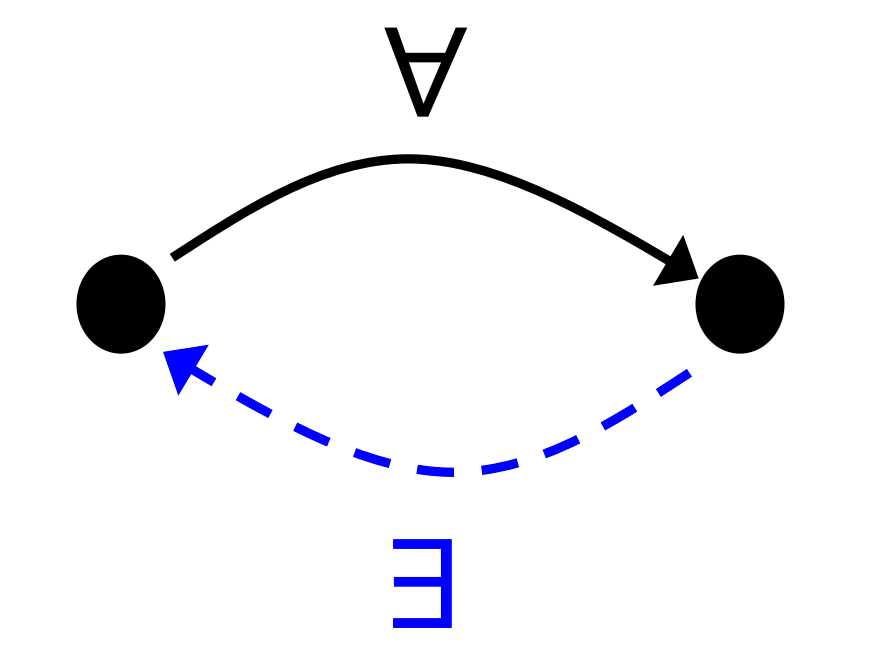
Symmetric

Definition

$R$ is symmetric iff for all elements $x$ that is related to $y$, $y$ is also related to $x$ $\forall x,y\in A(xRy\Rightarrow yRx)$

Not Symmetric

Negation of definition of symmetric $\exists x,y\in A(xRy\wedge y/Rx)$

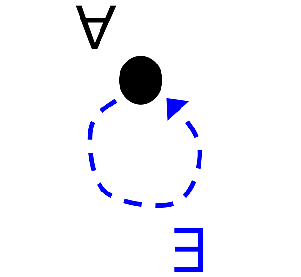
Antisymmetric

There does not exist elements $x,y$ where $x\ne y$ $x$ is related to $y$ and $y$ is related to $x$ Let $R$ be a relation on set $A$. $R$ is antisymmetric iff $\forall x,y\in A(xRy\wedge yRx\Rightarrow x=y)$

Different from not symmetric

• Not symmetric
  • At least one pair of elements is only related one way
• Asymmetric
  • Not a single pair of elements are related “two-way”, including two of the same element (i.e. no element is related to itself)
• Antisymmetric
  • Not a single pair of elements are related “two-way”

Asymmetric

$\forall x,y\in A(xRy\Rightarrow y/Rx)$

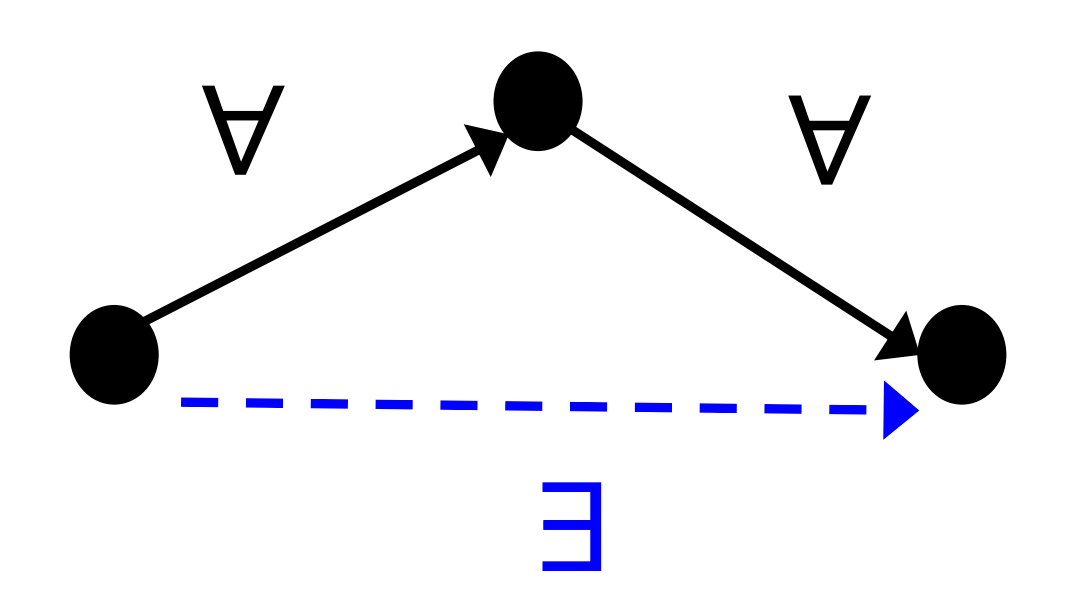
Transitive

Definition

$R$ is transitive iff for all elements $x$ that is related to $y$, and $y$ is related to $z$, $x$ is related to $z$ $\forall x,y,z\in A(xRy\wedge yRz\Rightarrow xRz)$

Transitive Closure

The transitive closure of a relation $R$, denoted as $R^t$, is the smallest superset of $R$ that is transitive i.e. To find $R^t$, add the least number of arrows to the directed graph of $R$ to make it transitive Note: when trying to find the transitive closure, keep checking for transitivity after each round of adding arrows Formally, it satisfies all the following:

1. $R^t$ is transitive
2. $R\subseteq R^t$
3. If $S$ is any other transitive relation that contains $R$ ($R\subseteq S$), then $R^t\subseteq S$
   • This means that $R^t$ is the smallest possible relation that is transitive

Example

Set Relation Properties 2024-10-04 02.56.54.excalidraw

⚠ Switch to EXCALIDRAW VIEW in the MORE OPTIONS menu of this document. ⚠ You can decompress Drawing data with the command palette: ‘Decompress current Excalidraw file’. For more info check in plugin settings under ‘Saving’

Excalidraw Data

Text Elements

Embedded Files

cbab65d6da187952222c5b0a286ec6ae3bf5e847: $R$

1e4bb51a12f788d49cec5e422dae640587999f05: $R^t$

95c5e3e3e5745bb8853e43e00feaabf3653d520d: image_1.png

4dbe37140d70d8134521bd5e2738f6238f412955: image_2.png

Link to original

Relation Induced by a Partition

Given a partition $\mathcal{C}$ of a set $A$, the relation $R$ induced by the partition is defined on $A$ as: $\forall x,y\in A$, $xRy\iff \exists$ a component $S$ of $\mathcal{C}$ such that $x,y\in S$ A partition is the same as an Equivalence Relations, but from different perspectives.

Properties

A relation induced by a partition is reflexive, symmetric and transitive

Example

Let set $A=\{0,1,2,3,4\}$ Let partition of the set $\mathcal{C}=\left\{\{0,1,2\},\{3\},\{4\}\right\}$ Relation induced by the partition is: $0R0,0R1,0R2,1R0,1R1,1R2,2R0,2R1,2R2,3R3,4R4$

Relation Diagrams

Arrow Diagram

Let $A=\{1,2,3\}$ and $B=\{1,3,5\}$. Define relations $S$ and $T$ from $A$ to $B$ as follows: $\forall (x,y)\in A\times B$, $(x,y)\in S\iff x<y$ $T=\{(2,1),(2,5)\}$

Set Relations 2024-10-03 17.49.49.excalidraw

⚠ Switch to EXCALIDRAW VIEW in the MORE OPTIONS menu of this document. ⚠ You can decompress Drawing data with the command palette: ‘Decompress current Excalidraw file’. For more info check in plugin settings under ‘Saving’

Excalidraw Data

Text Elements

1

2

3

1

3

5

S

1

2

3

1

3

5

T

Link to original

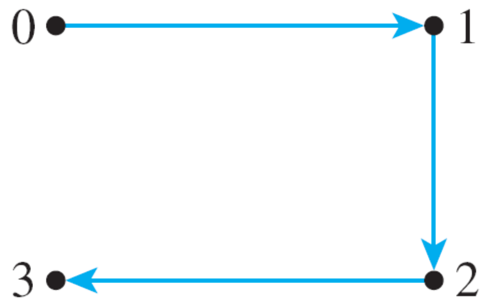
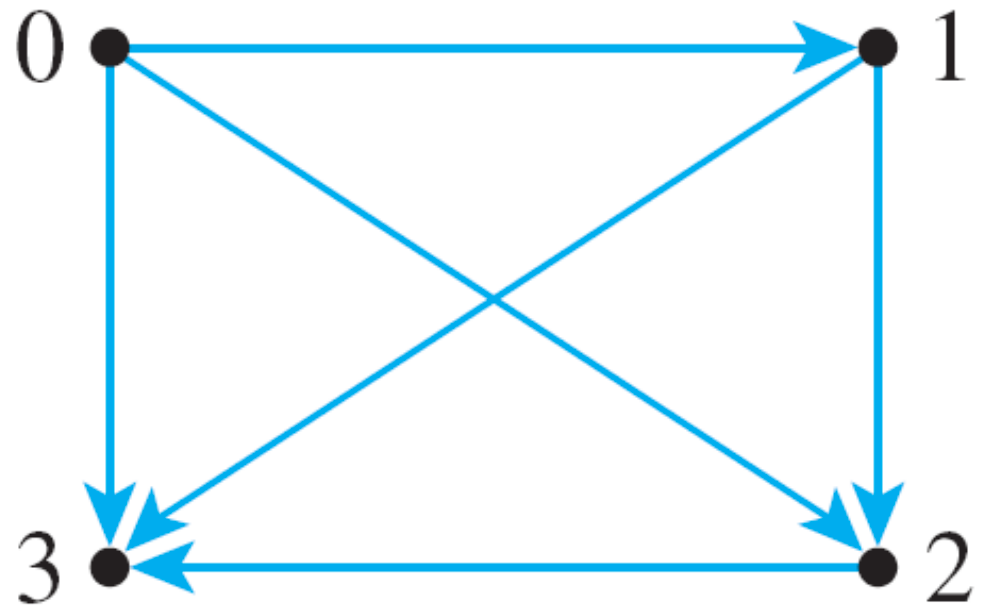
Directed Graph

Only for relations on a set. Let $A=\{3,4,5,6\}$, and define $R$ on $A$ as: $\forall x,y\in A,xRy\iff 2|(x-y)$

Set Relations 2024-10-03 20.23.45.excalidraw

⚠ Switch to EXCALIDRAW VIEW in the MORE OPTIONS menu of this document. ⚠ You can decompress Drawing data with the command palette: ‘Decompress current Excalidraw file’. For more info check in plugin settings under ‘Saving’

Excalidraw Data

Text Elements

3

4

6

5

Link to original

Relation Composition

Definition

Let $A$, $B$ and $C$ be sets. Let $R\subseteq A\times B$ be a relation, and $S\subseteq B\times C$ be a relation. The composition of $R$ with $S$ ($R\circ S$) is the relation from $A$ to $C$ such that: $\forall x\in A,\forall z\in C\left(xS\circ Rz\iff \left(\exists y\in B(xRy\wedge ySz)\right)\right)$ i.e. $x\in A$ and $z\in C$ are "$S\circ R$" related iff there s a “path” from $x$ to $z$ via some intermediate element $y\in B$ in the arrow diagram

Laws

Let $A$, $B$, $C$ and $D$ be sets. Let $R\subseteq A\times B$, $S\subseteq B\times C$ and $T\subseteq C\times D$ be relations.

Associative

$T\circ (S\circ R)=(T\circ S)\circ R=T\circ S\circ R$

Inverse

$(S\circ R{)}^{-1}=R^{-1}\circ S^{-1}$

Partial Order Relations

Definition

A relation is a partial order relation (or partial order) iff it is reflexive, antisymmetric and transitive. $\preccurlyeq$ is used to denote a partial order relation (it replaces $R$ in $aRb$, so $a\preccurlyeq b$), read ”$a$ is curly less than or equal to $y$“

Partially Ordered Set

A set $A$ is a partially ordered set or poset with respect to a partial order relation $R$ on $A$, denoted by $(A,R)$ A set with a partial order relation defined on it can be represented $(A,R)$ and be called a poset

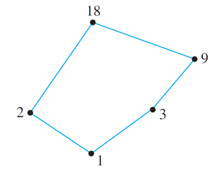
Hasse Diagram

Partial order relations can be represented as hasse diagrams

1. Start with a directed graph
2. Remove loops on nodes (because reflexive)
3. Arrange nodes such that all arrows are pointing up, then remove arrow heads (because antisymmetric)
4. Remove arrows that are implied by transitivity
   • If there is an arrow from $a$ to $b$ and $b$ to $c$, remove the arrow from $a$ to $c$
   • Keep repeating to remove as many arrows as possible

Example

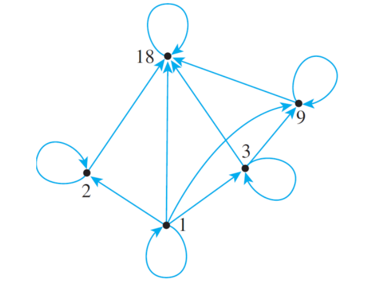
For the “divides” relation on set $A=\{1,2,3,9,18\}$

Partial Order Relations 2024-10-05 06.21.24.excalidraw

⚠ Switch to EXCALIDRAW VIEW in the MORE OPTIONS menu of this document. ⚠ You can decompress Drawing data with the command palette: ‘Decompress current Excalidraw file’. For more info check in plugin settings under ‘Saving’

Excalidraw Data

Text Elements

Directed Graph

Hasse Diagram

Embedded Files

200bb00677aa83342ccef1087c52e673c454aa82: image.png

acb4d4eb3d78d42155a9149398dea983c5eba8d5: image_0.png

Link to original

Formal Definition

Let $\preccurlyeq$ be a partial order on a set $A$. A Hasse diagram of $\preccurlyeq$ satisfies the following condition for all distinct $x,y,m\in A$: If $x\preccurlyeq y$ and no $m\in A$ is such that $x\preccurlyeq m\preccurlyeq y$, then $x$ is placed below $y$ with a line joining them, else no line joins $x$ and $y$

Analogy

Putting on socks and shoes (ignore reflexivity)

• left sock must go on before left shoe, same for right
• but whether the left or right sock goes on first does not matter
• whether the left shoe goes on before the right sock does not matter
• left sock $\preccurlyeq$ left shoe
• right sock $\preccurlyeq$ right shoe
• the order is “partial” because there may not be an order between certain elements
• left sock and right sock are not comparable

Common Examples

• The “divides” relation, $|$, on a set of positive integers
• $\le$ on a set of real numbers
• $\subseteq$ on a set of sets

Properties of Poset Elements

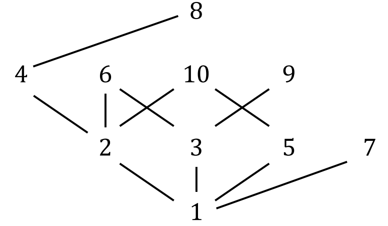
Suppose $\preccurlyeq$ is a partial order relation on a set $A$ For example, the hasse diagram of $|$ on $A=\{1,2,\dots ,10\}$

Comparability

Elements $a$ and $b$ of $A$ are said to be comparable iff either $a\preccurlyeq b$ or $b\preccurlyeq a$. Otherwise, $a$ and $b$ are noncomparable Hasse diagram: Comparable means having a path between the elements that only goes up In the example $2$ and $8$ are comparable, but $5$ and $9$ are not

Compatibility

Elements $a$ and $b$ of $A$ are said to be compatible iff there exists $c\in A$ such that $a\preccurlyeq c$ and $b\preccurlyeq c$
Hasse diagram: The elements have have a path upwards to the same elements
In the example, $1$ and $8$ , $2$ and $3$ are compatible but $3$ and $5$ are not

Maximal Element

Element $c$ of $A$ is a maximal element of $A$ iff $\forall x\in A$, either $x\preccurlyeq c$ or $x$ and $c$ are noncomparable $\forall x\in A(c\preccurlyeq x\Rightarrow c=x)$ Hasse diagram: There are no lines upward from the element In the example $6,7,8,9,10$ are the maximal elements

Minimal Element

Element $c$ of $A$ is a minimal element of $A$ iff $\forall x\in A$, either $c\preccurlyeq x$ or $x$ and $c$ are noncomparable $\forall x\in A(x\preccurlyeq c\Rightarrow c=x)$ Hasse diagram: There are no lines downward from the element In the example $1$ is the maximal elements

Largest Element

Element $c$ of $A$ is the largest element of $A$ iff $\forall x\in A(x\preccurlyeq c)$ A largest element is always also maximal Note: largest element = greatest element = maximum Hasse diagram: There is a path downwards to all other elements In the example there is no largest element

Smallest Element

Element $c$ of $A$ is the smallest element of $A$ iff $\forall x\in A(c\preccurlyeq x)$ A smallest element is always also minimal Note: smallest element = least element = minimum Hasse diagram: There is a path upwards to all other elements In the example $1$ is the smallest element

Linearisation

Creating a Total Order Relations from a partial order, without violating the partial order relation Let $\preccurlyeq$ be a partial order on a set $A$. A linearisation of $\preccurlyeq$ is a total order ${\preccurlyeq }^{\ast }$ on $A$ such that $\forall x,y\in A(x\preccurlyeq y\Rightarrow x{\preccurlyeq }^{\ast }y)$

Example

For the “divides” relation on $\{1,2,3,9,18\}$ Linearisations will include:

• $1{\preccurlyeq }^{\ast }2{\preccurlyeq }^{\ast }3{\preccurlyeq }^{\ast }9{\preccurlyeq }^{\ast }18$
• $1{\preccurlyeq }^{\ast }3{\preccurlyeq }^{\ast }2{\preccurlyeq }^{\ast }9{\preccurlyeq }^{\ast }18$
• etc.

Kahn’s Algorithm

An algorithm that takes a finite set $A$ and a partial order $\preccurlyeq$ on $A$, and outputs a linearisation ${\preccurlyeq }^{\ast }$ of $\preccurlyeq$ Informally:

1. Find the a minimal element of $A$
2. Remove the element from $A$
3. Repeat until $A=\varnothing$
4. The linearisation is the elements that were removed, in the order of removal

Total Order Relations

If $R$ is a partial order relation on set $A$, and for any two elements $x$ and $y$ in $A$, either $xRy$ or $yRx$, then $R$ is a total order relation (or total order) on $A$ $R$ is a total order iff $R$ is a partial order and $\forall x,y\in A(xRy\vee yRx)$ Also called a linear order

Example

The $\le$ relation on $\mathbb{Q}$ is a total order because $\forall x,y\in \mathbb{Q}(x\le y\vee y\le x)$

Well-Ordered Set

Let $\preccurlyeq$ be a total order on a set $A$. $A$ is well-ordered iff every non-empty subset of $A$ contains a smallest element $\forall S\in \mathcal{P}(A),S\ne \varnothing \Rightarrow (\exists x\in S\forall y\in S(x\preccurlyeq y))$

Equivalence Relations

A relation is an equivalence relation iff it is reflexive, symmetric and transitive. $\sim$ is commonly used to denote an equivalence relation (it replaces $R$ in $aRb$, so $a\sim b$) This is the same as a partition, but from a different perspective

Equivalence Class

The equivalence class of an element is the component of the partition that contains the element e.g. Partition $\mathcal{C}=\{\{1,2,3\},\{4\}\}$, the equivalence class of $1$, denoted $[1]$ is $\{1,2,3\}$ Formally, Suppose $A$ is a set and $\sim$ is an equivalence relation on $A$. For each $a\in A$, the equivalence class of $a$, denoted $[a]$, called the class of $a$ for short, is the set of all elements $x\in A$ such that $a$ is $\sim$-related to $x$. Symbolically, $[a{]}_{\sim }=\{x\in A:a\sim x\}$

Lemma Rel.1 Equivalence Classes

Let $\sim$ be a equivalence relation on a set $A$. The following are equivalent for all $x,y\in A$.

• $x\sim y$
• $[x]=[y]$
• $[x]\cap [y]\ne \varnothing$

Set of equivalence classes

For set $A$ and equivalence relation $\sim$ on $A$, the set of all equivalence classes with respect to $\sim$ is denoted $A/\sim$ (“the quotient of $A$ by $\sim$“) $A/\sim =\{[x{]}_{\sim }:x\in A\}$ This is a partition of $A$ (Theorem Rel.2)

Theorem Rel.2

Equivalence classes form a partition Let $\sim$ be an equivalence relation on set $A$, then $A/\sim$ is a partition of $A$

Common Example: Congruence Relations

Congruence

Let $a,b\in \mathbb{Z}$ and $n\in {\mathbb{Z}}^{+}$ $a$ is congruent to $b$ modulo $n$ iff $n|(a-b)$ ($a-b$ is divisible by $n$) can be written as $a\equiv b\mathrm{mod}n$

Congruence Relation

Congruence modulo $n$ (mod-$n$) relation $R$: $\forall x,y\in \mathbb{Z}(xRy\iff n|(x-y))$
The quotient $\mathbb{Z}/{\sim }_n$ where ${\sim }_n$ is the congruence-mod-n relation on $\mathbb{Z}$ is denoted ${\mathbb{Z}}_n$

Properties

Congruence modulo $n$ relation is an Equivalence Relation, i.e. it splits the set of integers into partitions.

Divisibility

Definition

If $n$ and $d$ are integers and $d\ne 0$, then $n$ is divisible by $d$ iff $n$ equals $d$ times some integer

Notation

$d|n$ means ”$d$ divides $n$”, if $n,d\in \mathbb{Z}$ and $d\ne 0$ $d|n\iff \exists k\in \mathbb{Z}$ such that $n=dk$

Quotient-remainder Theorem

Given any integer $n$ and positive integer $d$, there exist unique integers $q$ and $r$ such that $n=dq+r$ and $0\le r<d$ $\frac{n}{d}=q$ , with remainder $r$

Example Use

let: $T_0=n\in \mathbb{Z}:n=3k\text{, for some integer }k,$ $T_1=n\in \mathbb{Z}:n=3k+1\text{, for some integer }k,$ $T_2=n\in \mathbb{Z}:n=3k+2\text{, for some integer }k$ Is $\{T_0,T_1,T_2\}$ a partition of $\mathbb{Z}$?

Yes. By the quotient-remainder theorem, every integer $n$ can be written in exactly one of the three forms: $n=3k$, $n=3k+1$, or $n=3k+2$ for some integer $k$. This means that $T_0,T_1,T_2$ are mutually disjoint and $\mathbb{Z}=T_0\cup T_1\cup T_2$

---

Functions

Function

A function $f$ from a set $X$ to a set $Y$, denoted $f:X\to Y$ is a relation that satisfies the following ($f$ is well-defined)

1. $\forall x\in X\exists y\in Y(x,y)\in f$
2. $\forall x\in X\forall y_1,y_2\in Y\left(\left((x,y_1)\in f\wedge (x,y_2)\in f\right)\to y_1=y_2\right)$ (all the $y$ in 1. is unique) or
   Let $f$ be a relation on sets $X$ and $Y$ i.e. $f\subseteq X\times Y$ . Then $f$ is a function from $X$ to $Y$ iff $\forall x\in X\exists !y\in Y(x,y)\in f$
   or
   $f:X\to Y=\{(x,y):(x,y)\in (X\times Y)\wedge b=f(a)\}$
   or $f:X\to Y=\{(x,y):(x,y)\in (X\times Y)\wedge \forall x\in X\exists !y\in Y(x,y)\in f\}$
   A function from $X$ to $Y$ is a mapping from each element of $X$ to exactly one element of $Y$
   i.e. in the function diagram, there is only one arrow coming out from every element of $X$ and every element of $X$ has an arrow coming out of it
   or
   A function $f:X\to Y$ is well-defined (exists), if it has the following property:
   $\forall x_1,x_2\in X(x_1=x_2\to f(x_1)=f(x_2))$

Definitions

• let $f:X\to Y$ be a function. $f(x)=y$ iff $(x,y)\in f$
  • $x\stackrel{f}{\to }y$
  • $f:x\mapsto y$
• $x$ is the argument of $f$
• $f(x)$ is the image of $x$ under $f$
• If $f(x)=y$ then $x$ is a preimage of $y$
• $X$ is the domain of $f$
• $Y$ is the co-domain of $f$
• range is all possible outputs of $f$, or the setwise image of $X$ under $f$
• two functions can be derived from $g:X\to Y$
  • $f:\mathcal{P}(X)\to \mathcal{P}(Y)$ is the setwise image of $g$
  • $f^{-1}:\mathcal{P}(y)\to \mathcal{P}(X)$ is the setwise preimage of $g$
  • if $A\subseteq X$, then let $f(A)=\{f(x):x\in A\}$
  • if $B\subseteq Y$, then let $f^{-1}(B)=\{x\in X:f(x)\in B\}$
  • $f(A)$ is the setwise image of $A$, and $f^{-1}(B)$ is the setwise preimage of $B$ under $g$
  • note: $f^{-1}$ here is not an inverse function although they have the same symbol. $f^{-1}(\alpha )$ can also be written $\text{setwise\_preimage}(f)(\alpha )$
  • e.g. $g:\mathbb{Z}\to \mathbb{Z}$ defined $g(x)=x^2\forall x\in \mathbb{Z}$ . $g(\{-2,0,2\})=\{4,0,4\}=\{0,4\}$ and $g^{-1}(\{0,1,2\})=\{-1,0,1\}$ because $g(0)=0;g(-1)=g(1)=1$ and $g^{-1}(\{2\})=\{\}$
  • Setwise preimage function always exists
• Order of a bijection is the number of times a function has to be composed with itself to result in the identity function
  • For a bijection $f:A\to A$ of order $n$ : $f\circ f\circ \dots \circ f_n=i{d}_A$

Equality of Functions

$f:A\to B$ and $g:C\to D$ are equal ($f=g$) iff:

1. $A=C$ and $B=D$ , and
2. $f(x)=g(x)\forall x\in A$

Properties of Functions

• An injection (or injective function)
  • one-to-one or $\forall x_1,x_2\in X(f(x_1)=f(x_2)\to x_1=x_2)$ or equivalently (contrapositive), $x_1\ne x_2\to f(x_1)\ne f(x_2)$
  • f is not injective iff $\exists x_1,x_2\in X(f(x_1)=f(x_2)\wedge x_1\ne x_2)$
• A surjection (or surjective function or “onto”)
  • all elements in the co-domain have an input that result in it (range = co-domain)
  • $\forall y\in Y\exists x\in X(y=f(x))$
• A bijection (or bijective function)
  • one-to-one correspondence (all elements in co-domain has exactly one item that results in it)
  • a function is bijective iff it is both injective and surjective
  • $\forall y\in Y\exists !x\in X(y=f(x))$
  • If a function has an inverse, then it is bijective
• Inverse
  • for $f:X\to Y$ , $g:Y\to X$ is an inverse of $f$ iff $\forall x\in X\forall y\in Y(y=f(x)\leftrightarrow x=g(y))$
  • inverse of $f$ is denoted $f^{-1}$
  • inverse functions are unique
  • There exists an inverse iff it is bijective (theorem 7.2.3)

Composing Functions

Let $f:X\to Y$ and $g:Y\to Z$
The composition of f and g, $g\circ f:X\to Z$ is defined as: $(g\circ f)(x)=g(f(x))\forall x\in X$
From tutorial 6 Q2, $(g\circ f{)}^{-1}=f^{-1}\circ g^{-1}$

Identity Functions

The identity function on a set $X$ , $i{d}_x$ , is the function from $X$ to $X$ defined by $i{d}_x(x)=x$ for all $x\in X$ let $f:X\to Y$ Theorem 7.3.1:

• $f\circ i{d}_x=f$
• $i{d}_x\circ f=f$

Inverse Function

Composing a function ith its inverse results in the identity function: Theorem 7.3.2 (let $f:X\to Y$)

Properties

• Composing a function with its inverse results in the identity function (Theorem 7.3.2). Let $f:X\to Y$
  • $f^{-1}\circ f=i{d}_x$
  • $f\circ f^{-1}=i{d}_y$
• Function composition is associative
  • for $f:A\to B$, $g:B\to C$ and $h:C\to D$, then $(h\circ g)\circ f=h\circ (g\circ f)$
• Function composition is not commutative
  • Apart from special cases, $g\circ f\ne f\circ g$
• If $f$ and $g$ are both injective, then $g\circ f$ is injective (Theorem 7.3.3)
• If $f$ and $g$ are both surjective, then $g\circ f$ is surjective (Theorem 7.3.4)

Functions on ${\mathbb{Z}}_n$

• ${\mathbb{Z}}_n$ is the set of equivalence classes on mod-$n$ Congruence Relations.
  • In terms of functions, it can be taken that the domain is bounded to $n$ integer values
• Addition and multiplication functions on ${\mathbb{Z}}_n$ are well-defined (the “same” input will result in the “same” output (mod-n))
  • Let $f$ be the $+$ mod-n function, and $[x]$ means $x$ mod $n$
    • $f$ is defined as $[x_1]f[y_1]=[x_1+y_1]$
    • well defined means: for all $n\in {\mathbb{Z}}^{+}$ and all $[x_1],[y_1],[x_2],[y_2]\in {\mathbb{Z}}_n$ : $[x_1]=[x_2]\wedge [y_1]=[y_2]\to [x_1]f[y_1]=[x_2]f[y_2]$
  • Same for multiplication

Representing Sequences and Strings

Sequence (infinite)

• A sequence $a_0,a_1,a_2\dots$ can be represented by a function $a$ whose domain is ${\mathbb{Z}}_{\ge 0}$ that satisfies $a(n)=a_n$ for all $n\in {\mathbb{Z}}_{\ge 0}$
  • Therefore, any function whose domain is ${\mathbb{Z}}_{\ge m}$ for some $m\in \mathbb{Z}$ represents a sequence
• Sequences can be denoted $A^{\infty }=Seq(A)=\exists n\in \mathbb{Z}\mathbb{Z}\to A$
  • i.e. all the elements of the sequence can be found in $A$

String (finite)

• A string is a finite sequence
• A string or word over set $A$ is an expression of the form $a_0{a}_1{a}_2\dots a_{l-1}$ where $l\in {\mathbb{Z}}_{\ge 0}$ and $a_0,a_1,\dots ,a_{l-1}\in A$
• $l$ is the length of the string. The empty string $\epsilon$ is the string of length $0$
• Strings can be denoted $A^{\ast }=Str(A)=\exists m\in \mathbb{Z},l\in {\mathbb{Z}}_{\ge 0}[m,m+l)\to A$
  • i.e. all the elements of the string can be found in $A$

Equality

• Sequences $a_0,a_1,a_2,\dots$ and $b_0,b_1,b_2,\dots$
  • if their corresponding elements are equal, or $a(n)=b(n)$ for every $n\in {\mathbb{Z}}_{\ge 0}$
• Strings
  • if their lengths are equal and their corresponding elements are equal, or $a_i=b_i$ for all $i\in \{0,1,\dots ,l-1\}$

---

Mathematical Induction

Used to prove properties for sequences (e.g. natural numbers)

Closed Form of Sequence

Closed form formula represents a sequence. It shows how the value of sequence term $a_k$ depends on $k$, e.g. $a_k=2k$ for all integers $k\ge 1$

Sequence Comprehension

Sequences can be represented: $a=[2k:k\in [\mathrm{1..}]]$
Type signature: $Seq(Q)=([1,\infty )\to Q)$

Recurrence Relation

A formula that relates each term $a_k$ to some of its predecessors
e.g. factorial:
0! = 1 n! = n (n-1)! for n $\ge$ 1

Recursive definition of set

For a set $S$,

• base clause: Specify that certain elements, called founders are in $S$
• recursion clause: Specify certain functions, called constructors, under which set $S$ is closed: if $f$ is a constructor and $x\in S$ , then $f(x)\in S$
• minimiality clause: Membership for $S$ can always be demonstrated by finitely many successive applications of the clauses above

Principle of MI (1PI)

Let $P(n)$ be a property that is defined for integers $n$ and let $a$ be a fixed integer. Suppose the following statements are true:

1. $P(a)$ is true.
2. For all integers $k\ge a$ , if $P(k)$ is true then $P(k+1)$ is true.
   Then the statement “for all integers $n\ge a,P(n)$” is true.

Formally

$P(a)$ $\forall k\ge a,P(k)\Rightarrow P(k+1)$ $\therefore \forall k\ge a,P(k)$

To use

To prove “Fol all integers $n\ge a$ , a property $P(n)$ is true”
Step 1 (basis step): Show that $P(a)$ is true
Step 2 (inductive step): Show that for all integers $k\ge a$ , if $P(k)$ is true, then $P(k+1)$ is true, by the following:
Suppose that $P(k)$ is true, where $k$ is any particular but arbitrarilty chosen integer with $k\ge a$ (This is called the inductive hypothesis)
Then, show that $P(k+1)$ is true.

Example

Prove that for all integers $n\le 3,2n+1<2^n$

1. Let $P(n)\equiv (2n+1<2^n),\forall n\in {\mathbb{Z}}_{\ge 3}$
2. Basis step: $2\cdot 3+1=7<8=2^3$ . Therefore, $P(3)$ is true.
3. Assume $P(k)$ is true for $k\ge 3$ . That is, $2k+1<2^k$
4. Inductive step: (to show P(k+1) is true) 4.1. $2(k+1)+1=2k+3=(2k+1)+2<2^k+2<2^k+2^k=2^{k+1}$ (because $2<2^k$ for all integers $k\ge 2$ ) 4.2. Therefore $P(k+1)$ is true
5. Therefore, $P(n)$ is true for all integers $n\ge 3$

Principle of Strong MI (2PI)

Let $P(n)$ be a property that is defined for integers $n$ and let $a$ and $b$ be fixed integers with $a\le b$ . Suppose these statements are true:

1. $P(a),P(a+1),\dots ,P(b)$ are all true (basis step)
2. For any integer $k\ge b$ , if $P(i)$ is true for all integers $i$ from $a$ through $k$ , then $P(k+1)$ is true ($P(a)\wedge P(a+1)\wedge \dots \wedge P(k)\Rightarrow P(k+1)$ ) (inductive step)
   Then the statement “for all integers $n\ge a,P(n)$ ” is true

Variation 1

If

1. $P(a),P(a+1),\dots ,P(b)$ hold
2. For every $k\ge a,P(k)\Rightarrow P(k+b-a+1)$ ($P(k)$ implies something further down)
   Then $P(n)$ holds for all $n\ge a$

Variation 2

If

1. $P(a),P(a+1),\dots ,P(b)$ hold
2. For every $k\ge b\exists ia\le i\le k,P(i)\Rightarrow P(k+1)$ ($P(i)$, where $a\le i\le k$ implies $P(k+1)$)
   Then $P(n)$ holds for all $n\ge a$

Example

Prove that any whole amount \geq \12$canbeformedbyacombinationof$4 and $5 coins

1. Let $P(n)\equiv (n=4a+5b)$ , for some $a,b\in \mathbb{N},n\ge 12$
2. Basis step: Show that $P(12),P(13),P(14),P(15)$ hold: $12=4\cdot 3+5\cdot 0;13=4\cdot 2+5\cdot 1;$ (etc. not written here)
3. Assume $P(i)$ holds for $12\le i\le k$ given some $k\ge 15$
4. Inductive step: (To show $P(k+1)$ is true) 4.1. $P(k-3)$ holds (by induction hypothesis), so $k-3=4a+5b$ for some $a,b\in \mathbb{N}$ 4.2. $k+1=(k-3)+4=(4a+5b)+4=4(a+1)+5b$ 4.3. Hence, $P(k+1)$ is true
5. Therefore, $P(n)$ is true for $n\ge 12$

---

Cardinality

Pigeonhole Principle

Let $A$ and $B$ be finite sets. If there is an injection $f:A\to B$ , then $|A|\le |B|$ Contrapositive: Let $m,n\in {\mathbb{Z}}^{+}$ with $m>n$ . If $m$ pigeons are put into $n$ pigeonholes, then there must be (at least) one pigeonhole with (at least) two pigeons.

Dual Pigeonhole Principle

Let $A$ and $B$ be finite sets. If there is an surjection $f:A\to B$ , then $|A|\ge |B|$ Contrapositive: Let $m,n\in {\mathbb{Z}}^{+}$ with $m<n$ . If $m$ pigeons are put into $n$ pigeonholes, then there must be (at least) one pigeonhole with no pigeons.

Finite vs Infinite set

A set $S$ is said to be finite if it is empty, or there exists a bijection from $S$ to the set of positive integers from 1 to $n$ $\{1,2,3,...,n\}$
A set $S$ is said to be infinite if it is not finite

Cardinality

Finite Set

The cardinality of a finite set $S$, denoted $|S|$, is

1. 0 if $S=\varnothing$ or
2. $n$ if $f:S\to \{1,2,\dots ,n\}$ is a bijection
   Equality of cardinality of finite sets theorem For finite sets $A$ and $B$ : $|A|=|B|$ iff there is a bijection $f:A\to B$
   Any subset of a finite set is finite (contrapositive: any subset of a infinite set is infinite)

Infinite Sets

Given two sets $|A|$ and $|B|$ , $A$ is said to have the same cardinality as $B$ , written as $|A|=|B|$ , iff there is a bijection $f:A\to B$
note: we define what $|A|=|B|$ is without defining what $|A|$ or $|B|$ is
Another definition: Set $A$ is infinite iff there exists a set $B$ such that $(B\subseteq A)\wedge (B\ne A)\wedge (|B|=|A|)$ (A proper subset of $B$ has the same cardinality as $B$)

Properties of cardinality

The same-cardinality relation is an equivalence relation. For all sets $A$, $B$ and $C$

• Reflexive: $|A|=|A|$
• Symmetric: $|A|=|B|\to |B|=|A|$
• Transitive: $(|A|=|B|)\wedge (|B|=|C|)\to |A|=|C|$

Countability

A set is countable iff it is finite our countable infinite. Otherwise, it is uncountable.

Countably Infinite

Theorem 7.4.3: Any subset of any countable set is countable. (Contrapositive: Any set with an uncountable subset is uncountable.)
Lemma 9.4: Let $A$ and $B$ be countable infinite sets. Then $A\cup B$ is countable

Definition through bijection with ${\mathbb{Z}}^{+}$

“aleph zero” $={\aleph }_0=|{\mathbb{Z}}^{+}|$
A set $A$ having the same cardinality as ${\mathbb{Z}}^{+}$ is called a countably infinite set i.e. $|A|={\aleph }_0$
If sets $A_1,A_2,...,A_n$ are countably infinite, so is the cartesian product $A_1\times A_2\times \dots \times A_n$

Definition through sequence

An infinite set $B$ is countable iff there is a sequence $b_0,b_1,b_2,\dots \in B$ in which every element f $B$ appears (exactly once — whether this is included doesn’t matter) (this is equivalent to the above definition)

Example

${\mathbb{Z}}^{+}\times {\mathbb{Z}}^{+}$ is countable
Arrange the elements in a grid as shown:

(1,1)	(1,2)	(1,3)
(2,1)	(2,2)	(2,3)
(3,1)	(3,2)	(3,3)
We can count the ordered pairs following the diagonals: (1,1) → (1,2) → (2,1) → (1,3) → (2,2) → (3,1) etc. (sequence argument)
The function that represents this is $f(x,y)=\frac{(x+y-2)(x+y-1)}{2}+x$ (bijective function argument)
Therefore, ${\mathbb{Z}}^{+}\times {\mathbb{Z}}^{+}$ is countable.

Uncountable Infinite

A set is uncountable if it is impossible to find a bijection from that set to ${\mathbb{Z}}^{+}$ Theorem 7.4.2: The set of real numbers between 0 and 1, $(0,1)=\{x\in \mathbb{R}|0<x<1\}$ is uncountable
Proposition 9.3: Every infinite set has a countable infinite subset

Cantor’s diagonalization argument

(Prove the above by contradiction)

1. Suppose $(0,1)$ is countable
2. Since it is not finite, it is countable infinite
3. We list the elementns $x_{i}of(0,1)inasequenceasfollows:$x_1 = 0.a_{11}a_{12}a_{13}…a_{1n}…x_2 = 0.a_{21}a_{22}a_{23}…a_{2n}…x_3 = 0.a_{31}a_{32}a_{33}…a_{3n}……x_n = 0.a_{n1}a_{n2}a_{n3}…a_{nn}……$whereeach$a_{ij} \in {0,1,…,9}$ is a digit. (For numbers that have two representations 0.499… = 0.500…, we use only the latter representation)
4. Now, construct a number (from a diagonal of the above sequence) $d=0.d_1{d}_2{d}_3\dots d_n\dots$ such that

\begin{array}{ll} 1 & \text{if} a_{nn} \neq 1 \\ 2 & \text{if} a_{nn} = 1 \\ \end{array} \right.$$ 5. Note that $\forall n \in \mathbb Z^+, d_n \neq a_{nn}$ . Thus, $d \neq x_n, \forall n \in \mathbb Z^+$ 6. But clearly, $d \in (0, 1)$ . Hence, a contradiction. Therefore $(0,1)$ is uncountable # Well-ordering principle Every nonempty subset of $\mathbb{Z} _{\geq 0}$ has a smallest element --- # Counting & Probability # Random process/experiment When it takes place, one outcome from some set of outcomes is sure to occur, but it is impossible to predict with certainty which outcome that will be. ## Sample Space The set of all possible outcomes of a random process. An **event** is a subset of the sample space # Probability ## Probability Axioms Let $S$ be a sample space. A probability function $P$ from the set of all events in $S$ to the set of real numbers satisfies the following axioms for all events $A$ and $B$ in $S$, 1. $0 \leq P(A) \leq 1$ 2. $P(\varnothing) = 0$ and $P(S) = 1$ 3. If $A$ and $B$ are disjoint events ($A \cap B = \varnothing$), then $P(A\cup B) = P(A) + P(B)$ ## Probability of union of two events If $A$ and $B$ are any events in a sample space $S$ then $P(A\cup B) = P(A) + P(B) - P(A\cap B)$ ## Equally likely probability formula If $S$ is a finite sample space in which all outcomes are equally likely and $E$ is an event in $S$, then the probability of $E$, denoted $P(E)$ is $$P(E) = \frac{\text{Number of outcomes in }E}{\text{Total number of outcomes in }S} = \frac{|E|}{|S|}$$ ## Probability of complement of event $P(\bar A) = 1-P(A)$ ## Expected Value Suppos the possible outcomes of a probability experiment are real numbers $a_1,a_2,…,a_n$ which occur with probabilities $p_1,p_2,…,p_n$ respectively. The expected value of the experiment is: $\sum^n_{k=1}a_kp_k$ ## Conditional Probability Let $A$ and $B$ be events in a sample space $S$ . If $P(A) \neq 0$ then the conditional probability of $B$ given $A$ , denoted $P(B|A)$ is $\frac{P(A\cap B)}{P(A)}$ $P(A \cap B) = P(B|A) \cdot P(A)$ $P(A) = \frac{P(A\cap B)}{P(B|A)}$ ## Bayes’ Theorem Suppose that a sample space $S$ is a union of mutually disjoin events $B_1,B_2,…,B_2$ . Suppose $A$ is an event in $S$ and suppose $A$ and all the $B$ have non-zero probabilities. If $k$ is an integer with $1 \leq k \leq n$ then $$P(B_k | A) = \frac{P(A|B_k) \cdot P(B_k)}{P(A|B_1)\cdot P(B_1) + P(A|B_2) \cdot P(B_2) + ... + P(A|B_n) \cdot P(B_n)}$$ ## Independent Events For events $A$ and $B$ in sample space $S$ then they are indepent iff $P(A\cap B) = P(A) \cdot P(B)$ ### Mutually Independent For events $A$ $B$ and $C$ in a sample space $S$ . They are pairwise independent iff they satisfy conditons 1-3 below. They are mutually independent iff they satisfy all 4 conditions below. 1. $P(A\cap B) = P(A) \cdot P(B)$ 2. $P(A\cap C) = P(A) \cdot P(C)$ 3. $P(B\cap C) = P(B) \cdot P(C)$ 4. $P(A \cap B \cap C) = P(A) \cdot P(B) \cdot P(C)$ # Counting Theorem 9.1.1: If $m$ and $n$ are integers and $m \leq n$ then there are $n-m+1$ integers from $m$ to $n$ inclusive. ## Permutations A permutation of a set of objects is an ordering of distinguishable objects in a row (e.g. abc, acb, cba, bac, bca, cab) Theorem 9.2.2: The number of permutations of a set with $n$ ($n \geq 1$) elements is $n!$ Theorem 9.2.3: If $n$ and $r$ are integers and $1 \leq r \leq n$ then the number of r-permutations of a set of n elements $P(n,r) = n(n-1)(n-2)…(n-r+1)$ or $\frac{n!}{(n-r)!}$ ## r-combination let $n$ and $r$ be non-negative integers with $r \leq n$ An r-combination of a set of $n$ elements is a subset of $r$ of the $n$ elements. $\binom{n}{r}$ or n choose r, or $_nC_r$ denotes the number of subsets of size r (r-combinations) that can be chosen from a set of n elements. Theorem 9.5.1: $\binom{n}{r} = \frac{P(n,r)}{r!} = \frac{n!}{r!(n-r)!}$ ### Pascal’s Formula Theorem 9.7.1 $$\binom{n+1}{r} = \binom{n}{r-1} + \binom{n}{r}$$ ## Possibility trees ```text e.g. 2 coin tosses / \ Coin 1 H T / \ / \ Coin 2 H T H T ``` ## Multiplication Principle If an operations consists of $k$ steps and the first step can be performed in $n_1$ ways, second step in $n_2$ ways, $k^{\text{th}}$ step in $n_k$ ways, (regardless of how the other steps were performed), then the entire operation can be performed in $n_1 \times n_2 \times … \times n_k$ ways e.g. number of 4-digit numeric pins is $10 \times 10 \times 10 \times 10 = 1000$ e.g. number of 4-digit numeric pins without repeating digits is $10 \times 9 \times 8 \times 7$ ## Addition Rule If we have $m$ ways of doing something and $n$ ways of doing another thing and we cannot do both at the same time, then there are $m + n$ ways to choose one of these actions. Theorem 9.3.1: A finite $A$ equals the union of $k$ distinct mutually disjoint subsets $A_1,A_2,…,A_k$ Then $|A| = |A_1|+|A_2|+…+|A_k|$ ## Difference Rule Theorem 9.3.2: If $A$ is a finite set and $B \subseteq A$, then $|A\backslash B| = |A| - |B|$ ## Permutations with Indistinguishable Objects Suppose a collection consists of $n$ objects of which: $n_1$ are of type 1 and are indistinguishable from each other, …, $n_k$ are of type $k$ and are indistinguishable from each other The number of distinguishable permutations of the $n$ objects is $\binom{n}{n_1}\binom{n-n_1}{n_2}…\binom{n-n_1-n_2-…-n_{k-1}}{n_k} = \frac{n!}{n_1!n_2!…n_k!}$ ### Binomial Theorem For real numbers $a$ and $b$ and non-negative integers $n$ $$(a+b)^n = \sum^{n}_{k=0}\binom{n}{k}a^{n-k}b^k$$ ## r-combination with repetition Also known as a multiset of size $r$ A multiset of size $r$ chosen from a set $X$ of $n$ elements is an unordered selection of elements with repetition allowed. It is written as $[x_{i_1}, x_{i_2},…,X_{i_r}]$ Theorem 9.6.1: The number of multisets of size r that can be selected from a set of $n$ elements is $\binom{r+n-1}{r}$ This equals the number of ways $r$ objects can be selected from $n$ categories of objects with repetitions allowed ## Inclusion/Exclusion rule If $A$, $B$ and $C$ are finite sets, then $|A \cup B| = |A| + |B| - |A \cap B|$ $|A \cup B \cup C| = |A| + |B| + |C| - |A \cap B| - |A\cap C| - |B \cap C| + |A \cap B \cap C|$ ## Pigeonhole Principle 2 A function from one finite set to a smaller finite set cannot be injective ### Generalised For any function $f$ from a finite set $X$ with n elements to a finite set $Y$ with $m$ elements and for any positive integer $k$ if $k < n/m$ then there is some $y \in Y$ such that $y$ is the image of at least $k+1$ distinct elements of $X$ Contrapositive: For any funciton $f$ from a finite set $X$ with $n$ elements to a finite set $Y$ with $m$ elements and for any positive integer $k$, if for each $y \in Y, f^{-1}(\{y\})$ has at most $k$ elements, then $X$ has at most $km$ elements. ($n \leq km$) # Summary | | Order Matters | Order Doesn’t Matter | | ---------------------- | ------------- | -------------------- | | Repetition Allowed | $$n^k$$ | $$\binom{k+n-1}{k}$$ | | Repetition not Allowed | $$P(n,k)$$ | $$\binom{n}{k}$$ | --- # Graphs # Types of Graph ## Undirected Graph An undirected graph $G$ consists of 2 finite sets: a nonempty set of $V$ vertices and a set $E$ of edges, where each edge is associated with a set consisting of either one or two vertices called its **endpoints.** An edge is said to **connect** its endpoints. Two vertices that are connected to an edge are called **adjacent vertices** (vertices can be adjacent to themselves). An edge is said to be **incident on** each of its endpoints, and two edges incident on the same endpoint are called **adjacent edges.** Denoted $G = (V,E)$ where - $V = \{v_1, v_2,…,v_n\}$ is the set of vertices (or nodes) in $G$ - $E = \{e_1, e_2,…,e_k\}$ is the set of undirected edges in $G$ - An undirected edge $e$ connecting $v_i$ and $v_j$ is denoted $e=\{v_i,v_j\}$ ## Directed Graph Definition is same as [[#undirected-graph|Undirected Graph]], except $E$ is a set of ordered pairs, representing **directed edges.** An edge from $v$ to $w$ is $e=(v,w)$ ## Subgraph A graph $H$ is said to be a subgraph of $G$ iff every vertex in $H$ is also a vertex in $G$ , every edge in $H$ is also an edge in $G$ , and has the same endpoints as it has in $G$ ## Simple Graph An undirected graph that does not have any loops or parallel edges (no pair of vertices has two edges between them) ### Complete Graph A complete graph on $n$ vertices, $n > 0$, denoted $K_n$ is a simple graph with $n$ vertices and exactly one edge connecting each pair of distinct vertices. $K_n$ has $n(n-1) / 2$ edges. ## Bipartite Graph (or bigraph) is a simple graph whose vertices can be divided into two disjoin sets $U$ and $V$ such that every edge connects a vertex in $U$ to one in $V$ ### Complete Bitartite Graph A bigraph on two disjoint sets $U$ and $V$ such that every vertex in $U$ connects to every vertex in $V$ . If $|U| = m$ and $|V| = n$ , the complete bipartite graph is denoted as $K_{m,n}$ # Definitions ## Degree of Undirected Graph - Degree of vertex $v$, denoted deg($v$) is the number of edges that are incident on $v$ , with an edge that is a loop counted twice. - Total degree of $G$ is the sum of the degrees of all the vertices of $G$ ## Indegree and Outdegree of Directed Graph - Indegree of vertex $v$ denoted $deg^-(v)$ is the number of directed edges that end at $v$ - Outdegree of vertex $v$ denoted by $deg^+(v)$ is the number of directed edges that originate from $v$ - $\sum_{v\in V} deg^-(v) = \sum_{v\in V} deg^+(v) = |E|$ ## Traversing - Walk: a walk from $v$ to $w$ is a finite alternating sequence of adjacent vertices and edges of $G$ - It has the form $v_0e_1v_1e_2…v_{n-1}e_nv_n$ where $v_0 = v, v_n = w$ and for all $i \in {1,2,…,n}$ $v_i-1$ and $v_i$ are the endpoints of $e_i$ - The number of edges $n$ is the length of the walk - The **trivial walk** from $v$ to $v$ consists of the single vertex $v$ - Trail: a walk that does not contain a repeated edge - Path: a trail that does not contain a repeated vertex - Closed Walk: a walk that starts and ends at the same vertex - Cycle or circuit: a closed walk of length at least 3 that does not contain a repeated edge - Simple cycle or simple circuit: a circuit that does not have any other repeated vertex except its first and last - Cyclic: An undirected graph is cyclic if it contains a loop or cycle. Otherwise, it is acyclic ## Euler Circuit - An euler circuit for $G$ is a circuit that contains every vertex and traverses every edge of $G$ exactly once - An eulerian graph is a graph that contains an euler circuit - Theorem 10.2.2: If a graph has an Euler circuit, then every vertex of the graph has positive even degree (contrapositive: if some vertex of a graph has odd degree, then the graph does not have an euler circuit) - Theorem 10.2.3: If a graph $G$ is connected and the degree of every vertex of $G$ is a positive even integer, then $G$ has an euler circuit - Theorem 10.2.4: A graph $G$ has an euler circuit iff $G$ is connected and every vertex of $G$ has positive even degree ## Euler Trail/path - An euler trail/path from $v$ to $w$ is a sequence of adjacent edges and vertices that starts at $v$ , ends at $w$ , passes through every vertex of $G$ at least once, and traverses every edge of $G$ exactly once. (Euler circuit but doesn’t need to start and end at the same vertex) - Corollary 10.2.5: There is an euler trail from $v$ to $w$ iff $G$ is connected, $v$ and $w$ have odd degree, and all other vertices of $G$ have positive even degree ## Hamiltonian Circuit - A simple circuit that includes every vertex of $G$ (every vertex appears exactly once, except for the first and the last, which are the same) - Hamiltonian graph: a graph that contains a hamiltonian circuit - Proposition 10.2.6: If graph $G$ has a hamiltonian circuit, then it has a subgraph $H$ with the following properties - $H$ contains every vertex of $G$ - $H$ is connected - $H$ has the same number of edges as vertices - Every vertex of $H$ has degree 2 ## Connectedness - Two vertices of a graph are connected iff there is a walk from $v$ to $w$ - The graph $G$ is connected iff for any two vertices $v$ and $w$ in $G$ , there is a walk from $v$ to $w$ - A graph $H$ is a connected component of a graph $G$ iff all of the following: - The graph $H$ is a subgraph of $G$ - The graph $H$ is connected - No connected subgraph of $G$ has $H$ as a subgraph and contains edges or vertices that are not in $H$ (It is the biggest possible, contains as many edges and vertices as possible) - Lemma 10.2.1 - If $G$ is connected, then any two distinct vertices of $G$ can be connected by a path - If vertices $v$ and $w$ are part of a circuit in $G$ and one edge is removed from the circuit, then there still exists a trail from $v$ to $w$ in $G$ - If $G$ is connected and $G$ contains a circuit, then an edge of the circuit can be removed without disconnecting $G$ ## Handshake Theorem Theorem 10.1.1: The total degree of a graph $G$ is 2 times the number of edges of $G$ - The total degree of a graph is even - In any graph, there are an even number of vertices of odd degree # Matrix representation of graph Note: $a_{ij}$ represents the element at the ith row and jth column of A. A $m \times n$ matrix has m columns and n rows ## Adjacency Matrix Let $G$ be a directed graph with ordered vertices $v_1, v_2,…v_n$ The adjacency matrix of $G$ is the $n \times n$ matrix $A = (a_{ij})$ over the set of non-negative integers such that: $a_{ij} =$ the number of arrows from $v_i$ to $v_j$ for all $i,j = 1,2,…,n$ i.e. the element at the ith row and jth column is the number of edges from the ith vertex to the jth vertex Note: an adjacency matrix of an undirected graph is symmetric (about the top-left to bottom-right diagonal) ## Counting walks of length n Theorem 10.3.2: If $A$ is the adjacency matrix of a graph, the i j-th entry of $A^n$ is the number of walks of length $n$ connecting the ith and jth vertices of the graph. ## Matrix Operations ### Scalar Product The scalar product or dot product of the ith row of $A$ and jth column of $B$ (where the number of elements in both are the same) is the sum of the individual products ($a_{i1}b_{1j} + a_{i2}b_{2j} + ... + a_{in}b_{nj}$) ### Matrix multiplication The matrix product of $A$ and $B$ (number of cols in $A$ must be the same as the number of rows in $B$). The matrix product is a matrix $C$ where the element $c_{ij}$ is the scalar product of row i of matrix $A$ and column j of matrix $B$ ### Identity matrix The main diagonal is all 1s, the rest is 0. ### $n^{th}$ power of a matrix For matrix $A$ , $A^n = A A^{n-1}$ , so $A^3 = A(A A)$ # Isomorphism of graphs Let $G = (V_G,E_G)$ and $G' =(V_{G'}, E_{G'})$ be two graphs. $G$ is isomorphic to $G'$ , denoted $G \cong G'$ iff there exists bijections: $g: V_G \rightarrow V_{G'}$ and $h: E_G \rightarrow E_{G'}$ that preserve the edge-endpoint functions of $G$ and $G'$ in the sense that for all $v \in V_G$ and $e \in E_G$ , $v$ is an endpoint of $e \Leftrightarrow g(v)$ is an endpoint of $h(e)$ (The graphs have the same shape after re-arranging) Alternately: Let $G = (V_G,E_G)$ and $G' =(V_{G'}, E_{G'})$ be two simple graphs. $G$ is isomorphic to $G'$ iff there exists a permutation (function) $\pi : V_G \rightarrow V_{G'}$ such that $\{u,v\} \in E_G \Leftrightarrow \{\pi(u), \pi(v)\} \in E_{G'}$ Theorem 10.4.1: Graph isomorphism is an equivalence relation # Planar Graph A planar graph can be drawn on a two-dimensional plane without edges crossing ## Kuratowski’s Theorem A finite graph is planar iff it does not contain a subgraph that is a subdivision of the complete graph $K_5$ or the complete bigraph $K_{3,3}$ (subdivision: a graph that is made by placing a vertex along any edge to turn it into two edges) ## Euler’s Formula For a connected planar simple graph $G = (V,E)$ with $e=|E|$ and $v=|V|$ , if we let $f$ be the number of faces, then $f = e-v+2$ (a face is a region bound by edges of a planar graph when it is drawn without overlapping edges. note: the area outside the whole graph is counted as a face) --- # Trees # Definitions - A graph is said to be **circuit-free** iff it has no circuits - A simple graph is called a **tree** iff it is circuit-free and connected - Lemma 10.5.1: A non-trivial tree has at least one vertex of degree 1 (actually, it has at least two vertices of degree 1) - Theorem 10.5.2: Any tree with $n$ vertices ($n>0$) has $n-1$ edges. - Theorem 10.5.4: If $G$ is a connected graph with $n$ vertices and $n-1$ edges, then $G$ is a tree. - A **trivial tree** is a tree that consists of a single vertex - A simple graph is called a **forest** iff it is circuit free and not connected - **Terminal vertex or leaf & internal vertex**: If tree $T$ has only one or two vertices, then each is called a terminal vertex. If $T$ has at least 3 vertices, then a vertex of degree 1 in $T$ is called a terminal vertex and a vertex of degree greater than 1 is called an **internal vertex** # Rooted Tree - A rooted tree is a tree in which there is one vertex that is distinguished from the others and called the **root**. - The **level** of a vertex is the number of deges along the unique path between it and the the root. - The **height** of a rooted tree is the maximum level of any vertex of the tree. - **Children, Parents etc.** - The children of an internal vertex $v$ of a rooted tree are the vertices that are adjacent to $v$ and are one level further away from the root than v - If $w$ is a child of $v$ , then $v$ is called the parent of $w$ - Two distinct vertices that share the same parent are called **siblings** - Given two distinct vertices $v$ and $w$ , if $v$ lies on the unique path between $w$ and the root, then $v$ is an **ancestor** of $w$ and $w$ is a **descendant** of $v$ # Binary Tree A binary tree is a rooted tree in which every parent has at most two children. Each child is designated either a left child or a right child. The left subtree of vertex $v$ is the binary tree whose root is the left child, and consists of the left child and its descendants. (same for right subtree) Number of distinct binary trees with n nodes: $\frac{(2n)!}{(n+1)!n!}$ A full binary tree is a binary tree in which each parent has exactly two children. - Theorem 10.6.2: For non-negative integers $h$ , if $T$ is any binary tree with height $h$ and $t$ terminal vertices, then $t\leq 2^h$ (equivalently, $\log_2t\leq h$) ## Full binary tree theorem If $T$ is a full binary tree with $k$ internal vertices, then $T$ has a total of $2k+1$ vertices and has $k+1$ terminal vertices # Binary Tree Traversal ## Breadth-first seach (BFS) - Visit vertices level-by-level - At each level, visit vertices from left to right ## Depth-first seach (DFS) - Pre-order - Print the data of the root (or current vertex) - Traverse the left subtree by recursively (pre-order) - Traverse the right subtree by recursively (pre-order) - In-order - Traverse the left subtree recursively (in-order) - Print the data of the root (or current vertex) - Traverse the right subtree recursively (in-order) - Post-order - Traverse the left subtree recursively (post-order) - Traverse the right subtree recursively (post-order) - Print the data of the root (or current vertex) - “Trick”: - Pre-order: draw a dot on the left of the vertex, In-order: bottom between the branches, post-order: right - Trace a “path” around the “perimeter” of the whole tree counter-clockwise (take the vertices as circles and edges to have thickness) - Print the vertex data when we pass a dot # Spanning Trees A spanning tree for a graph $G$ is a subgraph of $G$ that contains every vertex of $G$ and is a tree - Proposition 10.7.1: - Every connected graph has a spanning tree - Any two spanning trees for a graph have the same number of edges ## Minimum spanning tree For a weighted graph (where each edge has a real number weight, and the total weight of all edges is the total weight of the graph), a minimum spanning tree for a connected weighted graph is a spanning tree that has the least possible total weight compared to all other spanning trees for the graph. Note: if $G$ is a weighted graph and $e$ is an edge of $G$ , then $w(e)$ denotes the weight of $e$ and $w(G)$ denotes the total weight of $G$ ## Kruskal’s Algorithm (to get MST) 1. Go through the edges of a graph in order of increasing weight 2. For each edge, add it to what will become the minimum spanning tree, provided that it will not create a circuit 3. After n-1 edges have been added, where n is the number of vertices of the graph, these edges, together with the vertices of the graph, form a minimum spanning tree for the graph Note: If multiple edges have the same weight, then the minimum spanning tree might not be unique ## Prim’s Algorithm (to get MST) 1. Pick a vertex to start, and add it to the tree 2. Find the next vertex to add to the tree by finding the vertex that is connected to the current tree by an edge with the lowest weight i.e. keep adding the lowest weight vertex to the tree until all vertices have been added